Table of Contents
Background
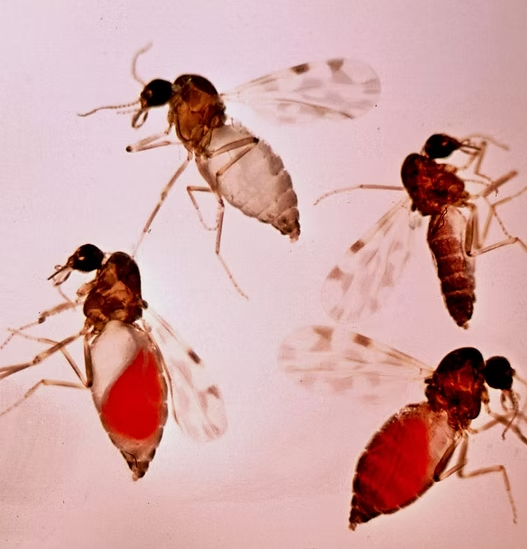
Biting midges of the family Ceratopogonidae (commonly called “no-see-ums”) represent a globally distributed insect group of over 5,000 species, many of which serve as vectors for dangerous pathogens affecting both humans and livestock. Culicoides sonorensis is the predominant and most well-characterized vector in North America, transmitting multiple arboviruses of significant economic and ecological importance:

The Challenge of Molecular Identification
Because comprehensive nuclear genomic resources are limited for most midge species, mitochondrial genomes have become the primary molecular resource for accurate species identification, phylogenetics, and population-level studies.
This is particularly critical for Culicoides sonorensis, which belongs to the variipennis complex: a group of morphologically cryptic, closely related species that are difficult to distinguish through morphological examination alone. Rapid and accurate identification is essential for surveillance programs aimed at monitoring virus distribution and predicting outbreak risk.
Mitogenomes offer a relatively compact (~15–17 kb), consistently structured, and rapidly evolving genomic target that can be sequenced cost-effectively from next-generation data. The mitochondrial protein-coding genes, which encode subunits of the oxidative phosphorylation machinery, are particularly useful for population-level differentiation because they accumulate substitutions at rates intermediate between slowly-evolving nuclear housekeeping genes and rapidly-mutating control regions.
Research Question:
Using de novo assembly of Illumina short reads from one individual C-sonorensis-F4, can we reconstruct a near-complete mitochondrial genome and identify genomic variants when compared to a second individual C-sonorensis-F2?
PIPELINE
FastQCTrimmomatic
    #!/bin/bash

    output_folder="data/processed/qc"
    data_folder="data/raw/q15-datafiles"

    # --- 1. FastQC : check quality before trimming --------
    module load fastqc
    fastqc -t 4 ${data_folder}/*.fq -o ${output_folder}

    # --- 2. Trimmomatic:  trim reads based on the following parameters --------------------

        # - ILLUMINACLIP: remove TruSeq3 adapters (2 mismatches; palindrome=30; simple=10)
        # - LEADING:3: trim very low-quality bases from 5' end (Q<3)
        # - TRAILING:20: trim low-quality bases from 3' end (Q<20)
        # - SLIDINGWINDOW:4:20: trim when 4-bp window avg quality <20
        # - MINLEN:50: discard reads <50 bp after trimming
        # Output: paired reads retained for assembly; unpaired reads saved separately

    module load trimmomatic
    out_folder="data/processed/trimm"

    # C. sonorensis F2
    # ------------------
    java -jar /apps/pkg/trimmomatic/0.39/trimmomatic-0.39.jar PE \
        ${data_folder}/C-sonorensis-F2_R1.fq \
        ${data_folder}/C-sonorensis-F2_R2.fq \
        ${out_folder}/F2R1_Trimmed_paired.fastq ${out_folder}/F2R1_Trimmed_unpaired.fastq \
        ${out_folder}/F2R2_Trimmed_paired.fastq ${out_folder}/F2R2_Trimmed_unpaired.fastq \
        ILLUMINACLIP:/apps/pkg/trimmomatic/0.39/adapters/TruSeq3-PE.fa:2:30:10 \
        LEADING:3 TRAILING:20 SLIDINGWINDOW:4:20 MINLEN:50

    # C. sonorensis F4
    # ------------------
    java -jar /apps/pkg/trimmomatic/0.39/trimmomatic-0.39.jar PE \
        ${data_folder}/C-sonorensis-F4_R1.fq \
        ${data_folder}/C-sonorensis-F4_R2.fq \
        ${out_folder}/F4R1_Trimmed_paired.fastq ${out_folder}/F4R1_Trimmed_unpaired.fastq \
        ${out_folder}/F4R2_Trimmed_paired.fastq ${out_folder}/F4R2_Trimmed_unpaired.fastq \
        ILLUMINACLIP:/apps/pkg/trimmomatic/0.39/adapters/TruSeq3-PE.fa:2:30:10 \
        LEADING:3 TRAILING:20 SLIDINGWINDOW:4:20 MINLEN:50


    # --- 3. FastQC: Check quality after trimming --------------------
    mkdir -p data/processed/qc/trimm
    fastqc -t 4 ${out_folder}/*_paired.fastq -o ${output_folder}/trimm
C-sonorensis-F4 dataset were assembled using SPAdes, which applies a de Bruijn graph assembly strategy optimized for short-read sequencing data. Assembly quality was evaluated using QUAST to assess assembly size and contig count.SPAdesQUAST
    #!/bin/bash

    data="data/processed/trimm"
    outfile="results/assembly"

    # --- 1. SPAdes: De Bruijn graph based assembly -----------
    module load spades
    spades.py \
        -1 ${data}/F4R1_Trimmed_paired.fastq \
        -2 ${data}/F4R2_Trimmed_paired.fastq \
        -o ${outfile}/spades_F4 \
        --isolate
        --careful

    # --- 2. QUAST: Evaluate genome assembly --------------------
    module load quast
    quast -o results/quast-out ${outfile}/spades_F4/contigs.fasta
C-sonorensis-F2 were aligned against the assembled F4 mitochondrial reference using BWA-MEM.BWA-MEMSAMtoolsBCFtools
    #!/bin/bash

    contigs="results/assembly/spades_F4/contigs.fasta"
    assembly="data/processed/assembly/F4_mt_ref.fasta"
    data="data/processed/trimm"
    out="results/variants/F2_F4.bam"

    # --- 1. Extract main contig from SPAdes output -----------------
    awk '/NODE_1_length_13603_cov_5.943010/{flag=1; print; next} /^>/{flag=0} flag' ${contigs} \
        > ${assembly}

    # --- 2. Index assembly sequence --------------------------------
    module load bwa samtools

    bwa index ${assembly}
    samtools faidx ${assembly}

    # --- 3. BWA-MEM: Align F2 reads to the F4 assembly reference -----
    bwa mem ${assembly} \
        ${data}/F2R1_Trimmed_paired.fastq \
        ${data}/F2R2_Trimmed_paired.fastq |
        samtools sort -o ${out}

    samtools index ${out}

    # --- 4. BCFtools: Variant call ----------------------------------
    module load bcftools

    bcftools mpileup -f ${assembly} ${out} | \
    bcftools call --ploidy 1 -mv -Ov -o results/variants/variants.vcf
NOTE:
Although Culicoides are diploid organisms, mitochondrial genomes are maternally inherited and exist in thousands of copies per cell with no recombination, functionally haploid. Variant calling was therefore performed with the
--ploidy 1flag in BCFtools, which assumes a single allele at each position. This is a critical parameter: calling with diploid settings would produce incorrect heterozygosity estimates and inflate false-positive variant rates.
Annotated genes were then compared against variant positions to determine which coding regions contained sequence variation.
GeSeqpython
    #!/usr/bin/env python3

    """
    analysis.py

    Parses GeSeq BLAT alignment results and a VCF file, then maps each variant
    to its corresponding gene region (or labels it as intergenic).

    Usage:
        python analysis.py
    """

    import sys
    from typing import Dict, List, Tuple

    # -----------------------------
    # Parsing
    # -----------------------------

    def parse_geseq(file: str) -> Dict[str, Tuple[int, int]]:
        """Parse a GeSeq BLAT output file and return deduplicated gene coordinates.

        Skips header, separator, and blank lines. For each valid alignment row,
        extracts the query name, query start/end positions, and derives the gene
        name from the target name (everything before the first underscore).

        When the same gene appears more than once (e.g. reverse-complement hits),
        only the longest span is retained.

        Args:
            file: Path to the GeSeq BLAT results text file.

        Returns:
            A dict mapping gene name -> (start, end) coordinate tuple,
            deduplicated to the longest hit per gene.
        """
        genes = []

        with open(file) as f:
            for line in f:
                if line.startswith("match") or line.startswith("-") or line.strip() == "":
                    continue
                parts = line.strip().split()
                if len(parts) < 17:
                    continue

                qstart = int(parts[11])
                qend   = int(parts[12])
                tname  = parts[13]
                gene   = tname.split("_")[0]   # gene name is before the first underscore

                genes.append((gene, qstart, qend))

        return _deduplicate_genes(genes)

    def _deduplicate_genes(genes: List[Tuple[str, int, int]]) -> Dict[str, Tuple[int, int]]:
        """Collapse duplicate gene hits by keeping the longest span per gene.

        Args:
            genes: List of (gene, start, end) tuples, possibly with duplicates.

        Returns:
            A dict mapping gene name -> (start, end) for the longest hit.
        """
        gene_dict = {}
        for gene, start, end in genes:
            length = end - start
            if gene not in gene_dict or length > (gene_dict[gene][1] - gene_dict[gene][0]):
                gene_dict[gene] = (start, end)
        return gene_dict

    def parse_vcf(vcf_file: str) -> List[Tuple[int, str, str]]:
        """Parse a VCF file and return a list of variants.

        Comment/header lines (starting with '#') are skipped. Each data row is
        expected to be tab-delimited with at least five columns conforming to the
        standard VCF layout: CHROM, POS, ID, REF, ALT, ...

        Args:
            vcf_file: Path to the VCF file.

        Returns:
            A list of (pos, ref, alt) tuples for every variant record.
        """
        variants = []

        with open(vcf_file) as f:
            for line in f:
                if line.startswith("#"):
                    continue
                parts = line.strip().split("\t")
                pos = int(parts[1])
                ref = parts[3]
                alt = parts[4]
                variants.append((pos, ref, alt))

        return variants

    # -----------------------------
    # Mapping
    # -----------------------------

    def map_variants(variants: List[Tuple[int, str, str]], genes: Dict[str, Tuple[int, int]]
    ) -> List[Tuple[int, str, str, str]]:
        """Assign each variant to a gene region based on its position.

        A variant is assigned to the first gene whose [start, end] span contains
        the variant position (inclusive). Variants that fall outside every gene
        region are labelled 'intergenic'.

        Args:
            variants: List of (pos, ref, alt) tuples from :func:`parse_vcf`.
            genes:    Dict of gene -> (start, end) from :func:`parse_geseq`.

        Returns:
            A list of (pos, ref, alt, gene) tuples with gene assignments.
        """
        results: List[Tuple[int, str, str, str]] = []

        for pos, ref, alt in variants:
            assigned = "intergenic"
            for gene, (start, end) in genes.items():
                if start <= pos <= end:
                    assigned = gene
                    break
            results.append((pos, ref, alt, assigned))

        return results

    # -----------------------------
    # Output
    # -----------------------------

    def print_results(mapped: List[Tuple[int, str, str, str]]) -> None:
        """Print mapped variants as a tab-separated table to stdout.

        Args:
            mapped: List of (pos, ref, alt, gene) tuples from :func:`map_variants`.
        """
        print("POS\tREF\tALT\tGENE")
        for pos, ref, alt, gene in mapped:
            print(f"{pos}\t{ref}\t{alt}\t{gene}")

    def print_summary(mapped: List[Tuple[int, str, str, str]]) -> None:
        """Print a per-gene variant count summary to stdout.

        Args:
            mapped: List of (pos, ref, alt, gene) tuples from :func:`map_variants`.
        """
        summary: Dict[str, int] = {}
        for _, _, _, gene in mapped:
            summary[gene] = summary.get(gene, 0) + 1

        print("\nVariant counts per gene:")
        for gene, count in sorted(summary.items()):
            print(f"  {gene}: {count}")
        print(f"\nTotal variants: {len(mapped)}")

    # -----------------------------
    # CLI entry point
    # -----------------------------

    def main() -> None:
        """Main entry point: parse arguments, run pipeline, and print output.
        """
        geseq_file = "GeSeq_results/GeSeqJob-20260506-220831_NODE_1_length_13603_cov_5.943010_blatX.txt"
        vcf_file = "pipeline/results/variants/variants.vcf"

        genes    = parse_geseq(geseq_file)
        variants = parse_vcf(vcf_file)
        mapped   = map_variants(variants, genes)

        print_results(mapped)
        print_summary(mapped)

    if __name__ == "__main__":
        main()
Results:
Assembly & Variant Summary
| Metric | Value |
|---|---|
| Total contigs from SPAdes | 2 |
| Primary contig length | 13,603 bp |
| Expected mtDNA size | 15,404 bp |
| Total variants identified | 34 |
| SNPs between individuals | 32 |
| INDELs between individuals | 2 |
| Variants in coding genes | 30 / 34 |
Assembly Contiguity
SPAdes produced two contigs from the F4 reads, with the primary contig spanning 13,603 bp, approximately 88% of the expected 15,404 bp mitochondrial genome size.

To investigate the missing region, trimmed F4 reads were remapped to the assembled contigs and reads near the contig boundaries were extracted for targeted local reassembly.
This produced a short secondary contig (~699 bp) characterized by very low sequencing coverage and repetitive AT-rich sequence motifs — consistent with the poorly assembling control region (also called the D-loop or A+T-rich region) described in the insect mitogenomics literature [1, 2]. This region is known to form secondary structures that resist short-read assembly, and its variants are therefore likely underrepresented in the dataset.
Variant Distribution Across Genes
Of the 34 total variants, 30 fell within annotated protein-coding genes. The highest density of variants was found in ND5, followed by CYTB, ND6, and COX2.
| Gene | Variant Count | Function |
|---|---|---|
| ND5 | 7 | NADH dehydrogenase subunit 5 |
| CYTB | 4 | Cytochrome b |
| ND6 | 4 | NADH dehydrogenase subunit 6 |
| COX2 | 4 | Cytochrome c oxidase subunit II |
| ND1, ND4, COX3 & others | 11 | Various OXPHOS components |
| Intergenic / control region | 4 | Non-coding / unannotated |
Key Findings & Biological Significance
Variants concentrate in OXPHOS genes. The majority of variants fall within genes encoding subunits of the oxidative phosphorylation (OXPHOS) complexes: particularly NADH dehydrogenase and cytochrome oxidase subunits. These genes are known hotspots of intraspecific variation in insect mitogenomes.
Control region underrepresented. The AT-rich control region could not be fully assembled, a well-documented limitation of short-read sequencing for this genomic feature. Long-read sequencing (PacBio or Nanopore) would resolve this region and provide a complete circular mitogenome.
Near-complete coverage achieved. At 88% of the expected genome size, the assembly is sufficient for gene annotation and population-level variant calling across all known protein-coding genes, providing a robust foundation for species identification.
Haploid calling was essential.
Explicitly specifying --ploidy 1 was critical to accurate variant identification. Treating the mitogenome as diploid would have generated spurious heterozygous calls and misrepresented the true SNP count between individuals.
Bioinformatics Tools:
| Tool | Purpose | Category |
|---|---|---|
| FastQC | Read quality assessment | QC |
| Trimmomatic | Adapter trimming & quality filtering | QC |
| SPAdes | De novo genome assembly (de Bruijn graph) | Assembly |
| QUAST | Assembly quality & contiguity metrics | Assembly |
| BWA-MEM | Short-read alignment to reference | Alignment |
| SAMtools | BAM sorting, indexing, and manipulation | Alignment |
| BCFtools | Variant calling and VCF filtering | Variant Calling |
| GeSeq | Mitochondrial genome annotation | Annotation |
References:
- Boore, J. L. (1999). Animal mitochondrial genomes. Nucleic Acids Research, 27(8), 1767–1780. https://doi.org/10.1093/nar/27.8.1767
- Cameron, S. L. (2014). Insect mitochondrial genomics: implications for evolution and phylogeny. Annual Review of Entomology, 59, 95–117. https://doi.org/10.1146/annurev-ento-011613-162007.
- Tillich, M. et al. (2017). GeSeq – versatile and accurate annotation of organelle genomes. Nucleic Acids Research, 45(W1), W6–W11. https://doi.org/10.1093/nar/gkx391